Limits and infinitesimals
Main articles: Limit of a function and Infinitesimal
Calculus is usually developed by working with very small quantities. Historically, the first method of doing so was by infinitesimals. These are objects which can be treated like real numbers but which are, in some sense, "infinitely small". For example, an infinitesimal number could be greater than 0, but less than any number in the sequence 1, 1/2, 1/3, ... and thus less than any positive real number. From this point of view, calculus is a collection of techniques for manipulating infinitesimals. The symbols dx and dy were taken to be infinitesimal, and the derivative dy/dx was simply their ratio.
The infinitesimal approach fell out of favor in the 19th century because it was difficult to make the notion of an infinitesimal precise. However, the concept was revived in the 20th century with the introduction of non-standard analysis and smooth infinitesimal analysis, which provided solid foundations for the manipulation of infinitesimals.
In the 19th century, infinitesimals were replaced by the epsilon, delta approach to limits. Limits describe the value of a function at a certain input in terms of its values at a nearby input. They capture small-scale behavior in the context of the real number system. In this treatment, calculus is a collection of techniques for manipulating certain limits. Infinitesimals get replaced by very small numbers, and the infinitely small behavior of the function is found by taking the limiting behavior for smaller and smaller numbers. Limits were the first way to provide rigorous foundations for calculus, and for this reason they are the standard approach.
Differential calculus[edit]
Main article: Differential calculus
Tangent line at (x, f(x)). The derivative f′(x) of a curve at a point is the slope (rise over run) of the line tangent to that curve at that point.
Differential calculus is the study of the definition, properties, and applications of the derivative of a function. The process of finding the derivative is called differentiation. Given a function and a point in the domain, the derivative at that point is a way of encoding the small-scale behavior of the function near that point. By finding the derivative of a function at every point in its domain, it is possible to produce a new function, called the derivative function or just the derivative of the original function. In mathematical jargon, the derivative is a linear operator which inputs a function and outputs a second function. This is more abstract than many of the processes studied in elementary algebra, where functions usually input a number and output another number. For example, if the doubling function is given the input three, then it outputs six, and if the squaring function is given the input three, then it outputs nine. The derivative, however, can take the squaring function as an input. This means that the derivative takes all the information of the squaring function—such as that two is sent to four, three is sent to nine, four is sent to sixteen, and so on—and uses this information to produce another function. (The function it produces turns out to be the doubling function.)
The most common symbol for a derivative is an apostrophe-like mark called prime. Thus, the derivative of the function of f is f′, pronounced "f prime." For instance, if f(x) = x2 is the squaring function, then f′(x) = 2x is its derivative, the doubling function.
If the input of the function represents time, then the derivative represents change with respect to time. For example, if f is a function that takes a time as input and gives the position of a ball at that time as output, then the derivative of f is how the position is changing in time, that is, it is the velocity of the ball.
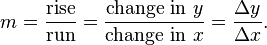
If a function is linear (that is, if the graph of the function is a straight line), then the function can be written as y = mx + b, where x is the independent variable, y is the dependent variable, b is the y-intercept, and:
This gives an exact value for the slope of a straight line. If the graph of the function is not a straight line, however, then the change in y divided by the change in x varies. Derivatives give an exact meaning to the notion of change in output with respect to change in input. To be concrete, let f be a function, and fix a point a in the domain of f. (a, f(a)) is a point on the graph of the function. If h is a number close to zero, then a + h is a number close to a. Therefore, (a + h, f(a + h)) is close to (a, f(a)). The slope between these two points is
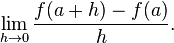
This expression is called a difference quotient. A line through two points on a curve is called a secant line, so m is the slope of the secant line between (a, f(a)) and (a + h, f(a + h)). The secant line is only an approximation to the behavior of the function at the point a because it does not account for what happens between a and a + h. It is not possible to discover the behavior at a by setting h to zero because this would require dividing by zero, which is undefined. The derivative is defined by taking the limit as h tends to zero, meaning that it considers the behavior of f for all small values of h and extracts a consistent value for the case when h equals zero:
Geometrically, the derivative is the slope of the tangent line to the graph of f at a. The tangent line is a limit of secant lines just as the derivative is a limit of difference quotients. For this reason, the derivative is sometimes called the slope of the function f.
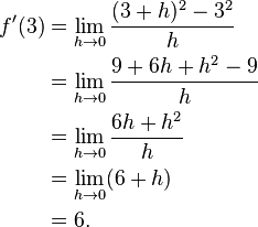
Here is a particular example, the derivative of the squaring function at the input 3. Let f(x) = x2 be the squaring function.